Understanding How Dimensionality Shapes Jet Stability in CFD

Introduction

One of the most important choices in any CFD workflow is dimensionality.
It often feels like a technical decision at first. Use 2D to save time, switch to 3D when needed.
But as I have worked on mixed convection, jet stability, and FCCVD reactor flows, it has become clear that dimensionality fundamentally reshapes the physics.

When we go from 3D to 2D, we are not just reducing the computational domain.
We are modifying the mathematical operator that governs the flow.
We are removing derivatives, velocity components, and entire instability pathways.

This post lays out, as clearly as possible, how 2D planar, 2D axisymmetric, and 3D models differ, what each can and cannot represent, and why these choices matter for asymmetric jets, buoyancy-driven vortices, and FCCVD transport.

Governing Equations and What Dimensionality Removes

Everything starts from the incompressible Navier–Stokes equations.

Continuity \(\nabla \cdot \mathbf{u} = 0\)

Momentum

Dimensional assumptions like
\(\frac{\partial}{\partial z}=0,\quad w=0,\) or
\(\frac{\partial}{\partial\theta}=0,\quad u_\theta=0,\) modify both the differential operators and the admissible solutions.

This restricts instability modes and symmetry-breaking pathways.

I like to think of dimensionality as a filter applied to the Navier–Stokes operator.

3D: The Full Physics and the Full Instability Spectrum

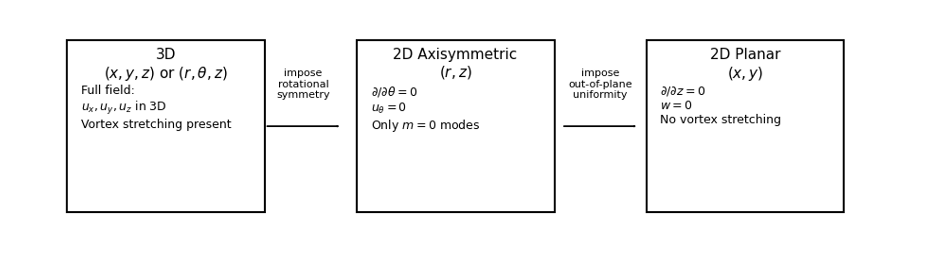
Figure 1. Dimensionality filtering applied to the Navier–Stokes equations.

In cylindrical coordinates ((r,\theta,z)),
the velocity field is \(\mathbf{u} = (u_r, u_\theta, u_z),\) and continuity becomes

The term that survives only in 3D is the vortex-stretching term: \(\boldsymbol{\omega}\cdot\nabla\mathbf{u}.\)

This drives:

• helical instabilities
• jet flapping
• azimuthal drift of buoyant plumes
• the classical turbulence cascade

The 3D stability spectrum contains all azimuthal modes
\(m = 0,\,1,\,2,\,\dots\)

This is why only 3D simulations can produce the classical (m=1) helical jet instability.

Axisymmetric 2D: The (m = 0) World

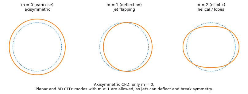
Figure 2. Axisymmetric modeling retains only (m=0) modes.

Axisymmetry imposes \(\frac{\partial}{\partial\theta}=0, \qquad u_\theta = 0.\)

Any perturbation of the form \(\tilde{u}(r,z)e^{im\theta}\) is removed for $(m\neq 0).$

Continuity reduces to

Axisymmetric CFD therefore cannot produce:

• helical motion
• flapping
• lateral instabilities
• buoyancy-induced azimuthal drift

It is excellent for mean-flow prediction, but cannot reveal asymmetric physics if the real flow is not symmetric.

Planar 2D: Limited Physics, But Free Symmetry Breaking

Planar simulations enforce \(\frac{\partial}{\partial z}=0,\qquad w=0.\)

Continuity becomes

Vorticity becomes a scalar, \(\omega = \frac{\partial v}{\partial x} - \frac{\partial u}{\partial y},\)

and is governed by \(\frac{D\omega}{Dt} = \nu\nabla^2\omega.\)

Because vortex stretching vanishes, \((\boldsymbol{\omega}\cdot\nabla)\mathbf{u} = 0,\) planar flows cannot generate 3D cascades.

But they can break symmetry in the plane, which is why a centered jet can deflect left or right.

The Pitchfork Bifurcation: Why 2D Jets Pick a Side

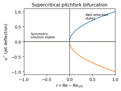
Figure 3. Supercritical pitchfork bifurcation for jet deflection.

Near the critical Reynolds number, the jet’s lateral displacement (u(t)) is governed by \(\frac{du}{dt} = r u - u^3,\) with
\(r \propto Re - Re_{\mathrm{crit}}\)

Steady states: \(u^* = 0,\qquad u^* = \pm\sqrt{r}\)

Stability follows from
\(\lambda = r - 3u^2\)

So:

• the centered jet $((u=0))$ is stable for $(r<0)$
• the two asymmetric jets $((u=\pm\sqrt{r}))$ are stable for $(r>0)$

This is the mathematical origin of Coandă attachment.
It is not numerical noise.

FCCVD and Buoyancy: Why 3D Is Almost Always Required

FCCVD reactors operate under extremely high thermal gradients, often
\(\Delta T \sim 800 - 1200\ \mathrm{K}\)

A useful measure of buoyancy is the Rayleigh number
\(Ra = \frac{g\beta \Delta T\, L^3}{\nu\alpha}\)

In FCCVD, (Ra) is typically large, which produces:

• asymmetric convection cells
• drifting buoyant plumes
• large recirculation regions
• lateral migration of catalyst particles

Buoyancy introduces azimuthal perturbations: \(\tilde{u}(r,z)e^{im\theta},\qquad m=1,2,\dots\)

Axisymmetric CFD cannot represent these.
Planar CFD can show symmetry breaking but cannot show full 3D plume drift.

These effects appear in both vertical and horizontal reactors.

Below is an example from a horizontal DI-FCCVD reactor.

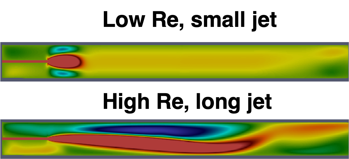
Figure 4. Buoyancy-driven mixed convection in a horizontal FCCVD reactor (adapted from Junnarkar et al., Carbon 2025).

The large plume drift and asymmetric recirculation correspond to $(m\ge1)$ modes and require 3D modeling.

Closing Thoughts

Dimensionality determines the physics a CFD model can express.
2D models are extremely useful for parameter sweeps and transition analysis, but they also remove entire instability families.

Once you view dimensionality as a filter on the Navier–Stokes equations, the differences between 2D and 3D simulations become much easier to interpret.

References

• [1] Effects of 2D Planar, Axisymmetric, and 3D Simulations on Jet Behavior and Stability
• [2] Hou, G. et al. Carbon nanotube reactor: Ferrocene decomposition…
• [3] Fearn, Mullin, Cliffe. Nonlinear flow phenomena in a symmetric sudden expansion.
• [4] Strogatz. Nonlinear Dynamics and Chaos.
• [5] Anderson. Computational Fluid Dynamics.
• [6] Additional unpublished FCCVD simulations
• [7] Private communication, Pasquali Research Group

Supporting Information: Mathematical Structure of Dimensional Reductions of Navier–Stokes

1. Full 3D Navier–Stokes (Cylindrical Coordinates)

Velocity:

Continuity:

Vorticity:

Vortex stretching term:

Nonzero only in 3D.

2. Axisymmetric Reduction

Constraints:

Continuity reduces to:

Linearized perturbations of the form

are only admissible for

Axisymmetric operator:

All helical (m = 1) and higher azimuthal modes are removed.

3. Planar Reduction

Constraints:

Continuity:

Scalar vorticity:

Vorticity transport:

No vortex stretching:

Planar 2D systems allow symmetry breaking in the plane but cannot develop 3D cascades.

4. Pitchfork Bifurcation Derivation

Let (u(t)) be the lateral jet displacement.

Center manifold reduction yields:

Steady states:

Jacobian:

Thus:

• (u^* = 0) is stable for (r < 0)
• (u^* = 0) is unstable for (r > 0)
• (u^* = \pm\sqrt{r}) are stable for (r > 0)

This is the canonical supercritical pitchfork bifurcation underlying 2D jet deflection.

5. Buoyancy Driven Mixed Convection in FCCVD

The relevant nondimensional group is the Rayleigh number:

FCCVD conditions typically give:

Buoyancy generates azimuthal perturbations of the form:

These modes:

• cannot appear in axisymmetric simulations ((m = 0) enforced)
• appear fully in 3D
• appear partially in planar 2D (but without 3D vortex stretching)

6. Summary Table