Beyond the Naked Eye: Building a Custom AI Pipeline for Carbon Nanotube Characterization
Published on: March 20, 2026
A deep dive into using Mask R-CNN, skeletonization, and perpendicular ray-casting to automatically measure nanotube diameters from TEM images - and why that matters for materials research.
TL;DR: An instance-segmentation pipeline (Detectron2 + Mask R-CNN) plus skeletonization and perpendicular ray-casting produces wall-to-wall CNT diameter measurements from TEM images in seconds; output CSV contains per-instance diameter (nm), per-image metadata, and confidence scores - enabling throughput impossible with manual Fiji measurements.
Key results (high level):
- 493 manually annotated CNT measurements converted to COCO-style training data.
- Mean outer diameter ~2.4 nm (dataset mean) with per-instance reporting (mean ± std).
- Inference produces per-image CSVs in seconds, enabling batch-level statistics.
The Challenge: A Bottleneck Built Into the Microscope
Transmission Electron Microscopy (TEM) is one of the most powerful tools a materials scientist has. At magnifications between 89,000x and 380,000x, you can resolve individual atomic planes, count walls in a multi-walled nanotube, and observe lattice defects that change macroscopic mechanical properties. For carbon nanotubes (CNTs), the outer diameter is not a cosmetic detail - it directly governs electronic band structure, van der Waals interactions between tubes, and ultimately, how a CNT-composite performs as an engineering material.
The problem is what happens after the image is taken.
Manual diameter measurement in Fiji/ImageJ looks deceptively simple: draw a line from one wall to the other and record the length. For a single well-separated nanotube this takes seconds. For real TEM frames with dense, overlapping bundles, measurement becomes slow, ambiguous, and subjective.
In practice, I was looking at:
- Dense bundles where five to fifteen individual tubes overlap, making it genuinely ambiguous where one tube ends and the next begins.
- Low-contrast walls caused by the projection of adjacent tube walls at similar orientations, or by slight defocus that spreads intensity across pixels.
- Background noise from the amorphous carbon support film, residual solvent contamination, or electron beam damage artifacts.
- Operator subjectivity - different researchers, or even the same researcher on different days, will draw that line slightly differently. For a tube with a true diameter of 2.4 nm, being off by one pixel at 185kx magnification (0.0168 nm/pixel) introduces an 0.7% error. Across hundreds of measurements, these biases accumulate and become statistically significant.
And that’s before accounting for scale. I had eight distinct sample batches (SP-58, SP-104, SP-107, SP-110, TL-58, TL-104, TL-107, TL-110), imaged at two accelerating voltages (80 kV and 300 kV) across magnifications ranging from 89kx to 380kx, producing 493 annotated CNT instances across 43 images. At a rate of two to three minutes per measurement in Fiji, that’s a full workday just to generate one round of ground truth. And each new synthesis batch means starting over.
I needed a way to make this scale. So I built one.
The Architecture: Why Instance Segmentation, Not Bounding Boxes
The first design decision - and the one that determines everything downstream - is how you represent a detected nanotube computationally.
The simplest approach is object detection with bounding boxes. A model like YOLO would output a rectangle around each CNT. Fast, well-understood, easy to train. But fundamentally wrong for this geometry. A nanotube in a TEM image is a long, thin, often curved object at arbitrary orientation. Its bounding box is dominated by its length, not its width. Worse, overlapping tubes in a bundle share bounding box area - meaning any width measurement derived from the box captures the bundle width, not the individual tube diameter. This was a non-starter.
The second option is semantic segmentation: classify every pixel as “nanotube” or “background.” This gives you the actual tube shape, which is progress. But it conflates all tubes in a bundle into a single connected region. You cannot extract individual diameters from a blob.
What I needed was instance segmentation: a separate binary mask for every individual nanotube detected in the image, allowing overlapping tubes to be treated as distinct objects even when their pixels spatially coincide.
This is exactly what Mask R-CNN provides.
The architecture (He et al., 2017) is a two-stage detector built on a Feature Pyramid Network (FPN) backbone. Stage one generates region proposals (candidate bounding boxes) via a Region Proposal Network (RPN). Stage two classifies each proposal and simultaneously predicts a binary segmentation mask at 28x28 pixel resolution, which is upsampled to the proposal size. The FPN backbone (here, a ResNet-50) extracts features at multiple scales simultaneously - critical when objects vary enormously in apparent size depending on magnification.
I implemented this using Detectron2 (Facebook AI Research), initialized with weights pretrained on the COCO dataset and fine-tuned on my CNT annotations. The framework handles the RPN, RoIAlign, and mask head architecture internally, which let me focus engineering effort on the parts that are genuinely domain-specific: anchor design, training resolution, and the diameter measurement algorithm.
One non-obvious configuration change was critical: custom anchor aspect ratios.
Standard COCO anchors use ratios of [0.5, 1.0, 2.0] - designed for objects like people, cars, and dogs that are roughly equidimensional. A CNT in a TEM image has an aspect ratio of 20:1 to 50:1. At 295kx magnification (0.0105 nm/pixel), a 2.4 nm diameter tube spans only ~23 pixels in width but may extend 300+ pixels in length. With standard anchors, the RPN simply never proposes a box that fits such an object - the detector is blind before it even tries to classify.
I replaced the standard ratios with:
cfg.MODEL.ANCHOR_GENERATOR.ASPECT_RATIOS = [
    [0.02, 0.05, 0.1, 0.2, 0.5, 1.0, 2.0, 5.0, 10.0]
] * 5  # applied at each FPN level
This single change was the difference between near-zero detections and a functional model.
The Methodology: From Raw TIF to Training-Ready Data
Ground Truth Creation: Reading the Fingerprints Left by Fiji
Before training a model, I needed to convert the existing manual annotations into a format the model could learn from. The annotations lived inside the TEM images themselves.
When a researcher uses Fiji to draw a measurement line and then flattens the image overlay, the colored line pixels are burned directly into the TIF file. The underlying TEM image is grayscale (R = G = B at every pixel), so any pixel with significantly unequal RGB channels is, by definition, part of an annotation rather than the TEM signal.
This is the core insight behind 01_parse_annotations.py. For each pixel (r, g, b), I compute a colorfulness score:
Pixels with colorfulness above a threshold of 40 are flagged as annotation pixels. Grayscale TEM pixels - even those with texture, noise, or varying brightness - will always score near zero, so they are naturally excluded.
Once the annotation mask is extracted, I use connected component labeling to isolate each individual drawn line. For each component, I fit a line through its pixel coordinates using Principal Component Analysis (PCA): the principal eigenvector gives the orientation of the line, and the projection range onto that eigenvector gives its length. This yields a centroid, an angle in degrees, and a length in pixels.
These image-derived measurements are then matched to the corresponding Fiji CSV file, which records the angle and length (in nanometers) for each drawn measurement. Matching is done greedily by angle similarity - angle is the most reliable signal because the pixel length estimate is sensitive to nm/pixel calibration uncertainty. The matched angle tolerance is ±45°, with length proximity used only as a tiebreaker with a weight of 0.2 relative to angle deviation.
After matching, a rectangular polygon mask is generated for each annotation, oriented along the CNT axis (perpendicular to the measurement line), with configurable width and length padding. These polygons become the instance segmentation masks for training.
Final match rate: 493 out of 493 annotations (100%).
COCO Conversion and the Train/Val Split
Detectron2 ingests annotations in COCO JSON format. The 02_coco_converter.py script converts the parsed annotations into this standard format and performs an 80/20 image-level train/validation split.
The final dataset:
| Split | Images | CNT Instances | Mean Diameter | Range |
|---|---|---|---|---|
| Train | 34 | 369 | 2.43 ± 0.54 nm | 1.22 - 5.18 nm |
| Val | 9 | 124 | 2.31 ± 0.44 nm | 1.13 - 3.93 nm |
The nm/pixel values are embedded in each COCO image record, derived from the magnification string in the filename, and span six calibrations:
| Magnification | nm/pixel |
|---|---|
| 89kx | 0.0350 |
| 115kx | 0.0270 |
| 145kx | 0.0214 |
| 185kx | 0.0168 |
| 230kx | 0.0135 |
| 295kx | 0.0105 |
| 380kx | 0.0082 |
Training: Memory Engineering as Much as Deep Learning
Training Mask R-CNN on a Colab T4 (15 GB VRAM) required memory engineering. The native images are 2048x2048, so I trained at 512x512 with batch size 1 and FP16 to fit the model. This stabilized memory use and enabled training, but requires a scale correction at inference (see Methods).
Training ran for 3,000 iterations with a base learning rate of 0.00025, warm-up over 200 iterations, and learning rate decay steps at iterations 2,010 and 2,670 (the standard 3x schedule for COCO-pretrained models).
Final training metrics at iteration 3,000:
- Total loss: ~0.70
loss_mask: ~0.48loss_rpn_cls: ~0.07loss_box_reg: ~0.09
A loss_mask of 0.48 (binary cross-entropy at the mask head) is reasonable for this dataset size. With 369 training instances of a single class, the model is working close to the data-limited regime. The mask quality is sufficient for diameter measurement - it does not need to be pixel-perfect, just accurate enough to capture the tube walls.
The Secret Sauce: Skeletonization and Perpendicular Ray-Casting
This is the part where “AI detected the nanotubes” becomes a quantitative scientific measurement.
A naive approach would be to take the bounding box of each predicted mask and use its minor axis as the diameter. This fails for the same reason bounding boxes failed at detection: a curved or tilted nanotube has a bounding box that overestimates its width, and a bundle of overlapping tubes compounds the error.
A slightly better approach would be to fit an ellipse to the mask and use its minor axis. This works for single, well-separated tubes at moderate curvature - but fails for tubes that are nearly parallel to the image edge, highly curved, or partially occluded, all of which are common in real bundle TEM images.
The approach I implemented is geometrically rigorous and robust to all these cases: skeletonization followed by perpendicular ray-casting.
Step 1: Medial Axis Skeletonization
Given the binary mask M for a detected nanotube instance (shape: H x W, True where the tube is), I compute the morphological skeleton using the Zhang-Suen thinning algorithm (implemented in skimage.morphology.skeletonize). The skeleton S is a one-pixel-wide representation of M that traces the centerline - the medial axis - of the tube.
Formally, the skeleton is the set of all points equidistant from at least two boundary points of M. For a straight tube of uniform width d, the skeleton is a single line segment running along the tube axis, and every skeleton point is at distance d/2 from the nearest boundary.
Step 2: Ordering Skeleton Points
The skeletonization outputs an unordered set of (y, x) pixel coordinates. To cast perpendicular rays, I need these ordered along the tube axis so I can estimate a local tangent at each sample point.
Ordering is done in two stages:
- PCA initialization: Project all skeleton points onto their first principal component. The point with the minimum projection value is selected as the traversal start.
- Nearest-neighbor traversal: From the start point, greedily visit the nearest unvisited skeleton point. If the nearest neighbor is more than 5 pixels away, traversal stops (indicating a fragmented or branched skeleton from bundle occlusion).
This produces an ordered sequence of skeleton pixels along the tube centerline.
Step 3: Perpendicular Ray-Casting
I sample N evenly-spaced points along the ordered skeleton (excluding the first and last, where boundary effects distort the tangent estimate). At each sample point, I compute the local tangent:
\[\hat{t}_i = \frac{p_{i+1} - p_{i-1}}{|p_{i+1} - p_{i-1}|}\]The perpendicular (normal) direction is obtained by rotating the tangent 90°:
\[\hat{n}_i = (-t_{i,y},\ t_{i,x}) \quad \text{(in image coordinates, where y is downward)}\]From each sample point, I cast two rays in opposite directions along the local normal, stepping one pixel at a time until each ray exits the mask. The exit distances in the two directions are d+ and d-.
The diameter at that sample point is:
\[d_i = d_+ + d_-\]This is the wall-to-wall distance measured perpendicular to the local tube axis - which is exactly what the researcher measured manually in Fiji, and exactly what the ground truth CSV records.
The reported diameter for a tube is the mean across all sample points, converted to nanometers using the magnification-derived nm/pixel calibration:
\[D_{\text{nm}} = \bar{d}_{\text{px}} \times \frac{\text{nm}}{\text{pixel}}\]The Scale Factor: An Important Implementation Detail
Because training was performed at 512px resolution on 2048x2048 pixel images, the predicted masks are returned at the inference resolution (512px), not the original image resolution. All pixel-space diameter measurements must therefore be multiplied by:
\[\text{SCALE} = \frac{2048}{512} = 4.0\]before converting to nm. The raw pixel measurements are stored in the output CSV (mean_diam_px) alongside the approximate nm/pixel values so that the nm conversion can be corrected independently if scale bar measurements are taken in Fiji for a specific image.
Visual Results
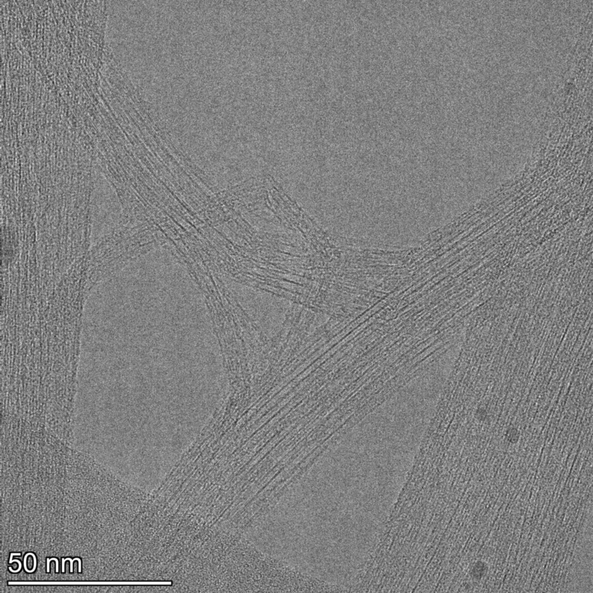
Figure 1 - Raw 2048x2048 TEM micrograph (example). Overlapping bundles and wall contrast vary across the frame.
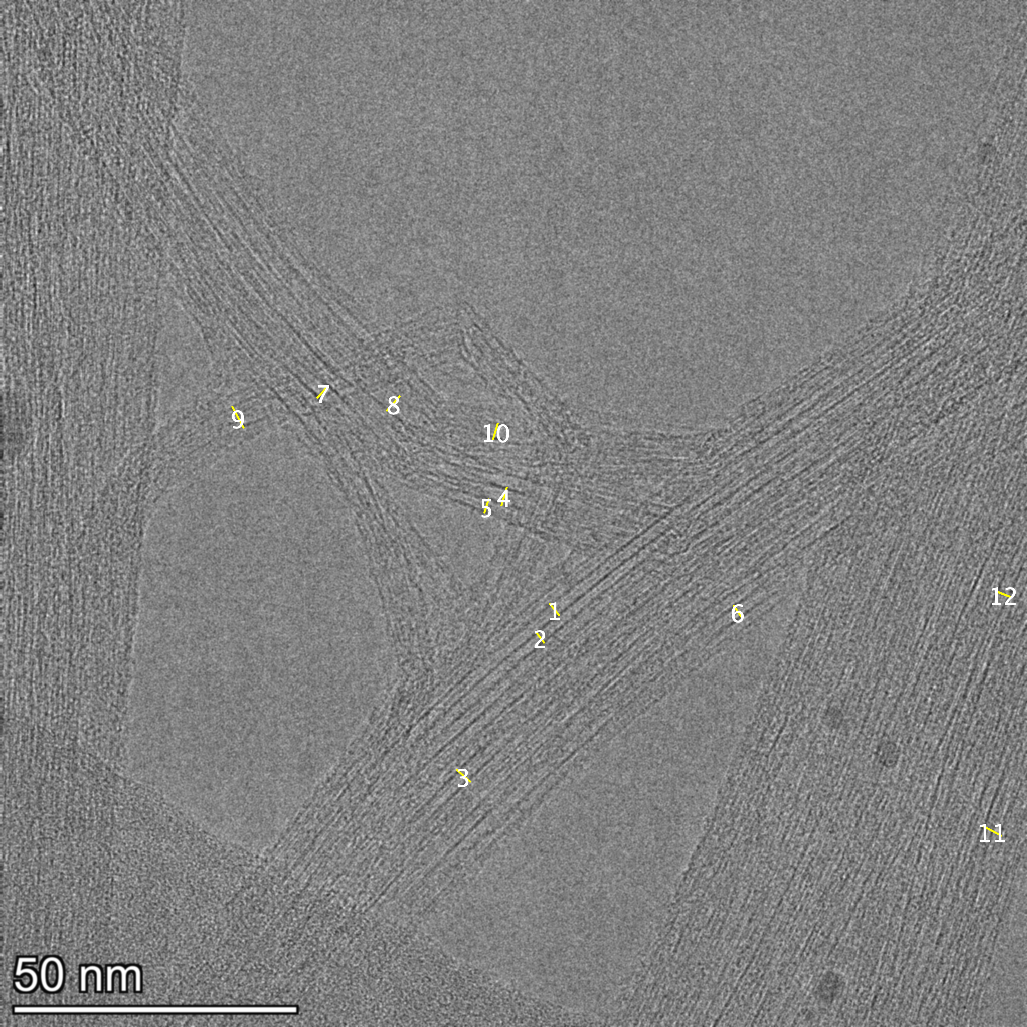
Figure 2 - Ground-truth annotations (Fiji) extracted from the annotated TIFF overlays used for training.
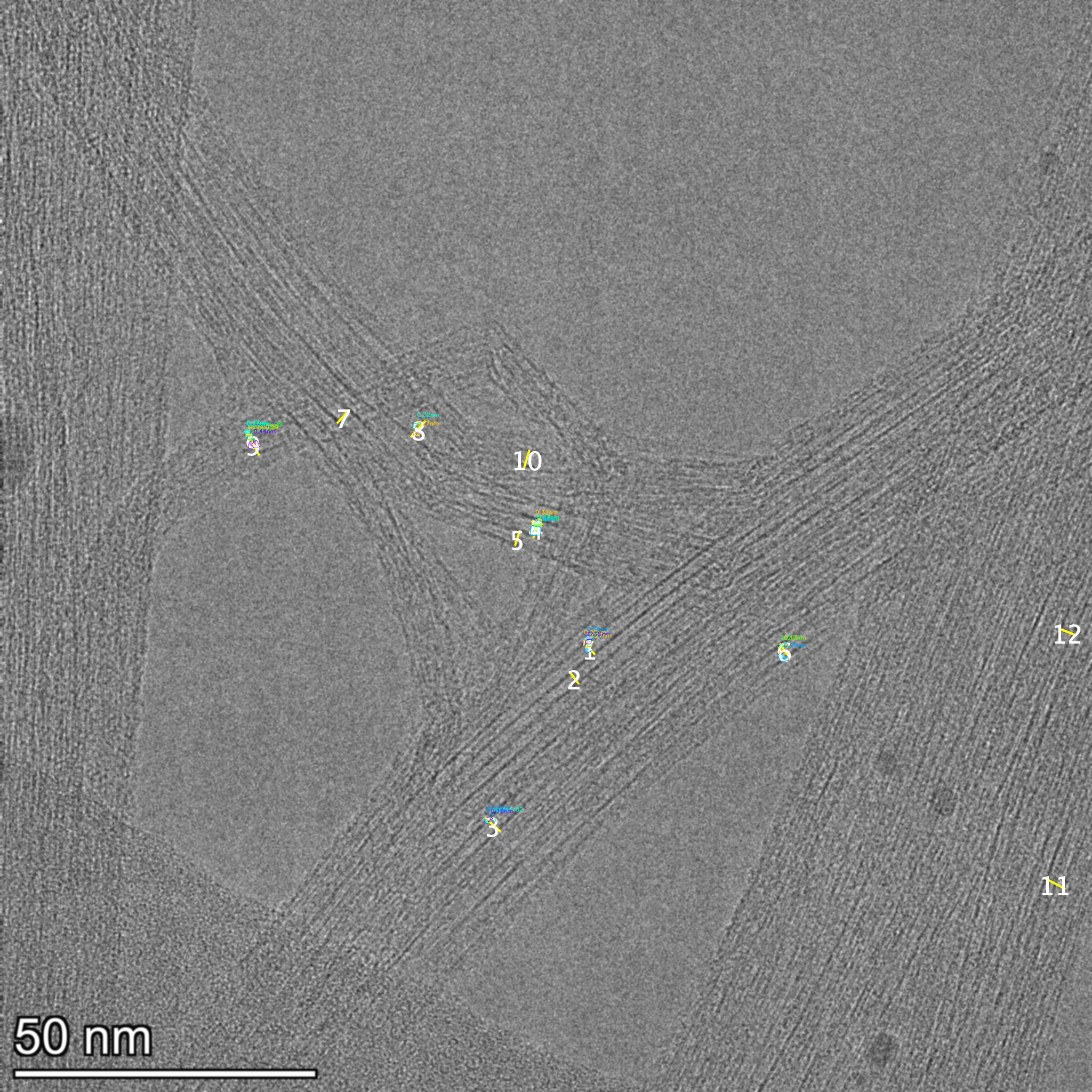
Figure 3 - Model predictions with instance masks and diameter labels (mean ± std in nm).
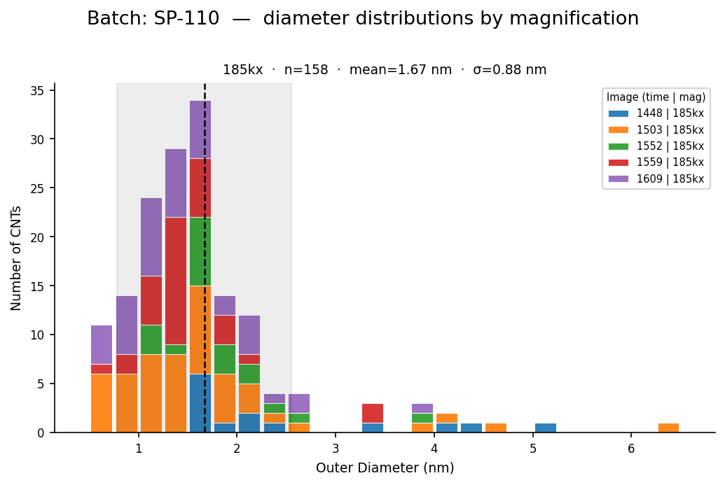
Figure 4 - Final per-batch diameter distribution (example). The pipeline outputs CSVs used to build these plots.
Current Limitations and Future Work
What the Model Gets Wrong - and Why
Dense bundle interiors. When five or more tubes are tightly packed and their walls are within 0.5 nm of each other, the inter-tube spacing approaches the pixel resolution at 295kx (0.0105 nm/pixel = ~1 Angstrom/pixel). The model tends to merge adjacent tubes in the bundle interior into a single instance, or miss them entirely. The perpendicular ray-casting algorithm can measure the merged region, but that measurement reflects the bundle diameter, not a single tube. These instances are filtered post-hoc by the diameter bounds (0.5-8.0 nm), but some remain.
Low-contrast images. At 80 kV accelerating voltage, the electron-matter interaction cross-section is higher, which actually improves contrast - but some samples show poor contrast due to thick or non-uniform support films. In these images, detection recall drops (fewer true positives at a given confidence threshold). Lowering the score threshold from 0.3 to 0.2 recovers detections but increases false positives.
Scale bar calibration. The nm/pixel values in the current pipeline are estimated from magnification strings in filenames. They are nominal factory-calibrated values. For the 300 kV images (TL-104 and TL-110 300kV batches), the actual pixel scale depends on the exact objective lens excitation used, which varies slightly between sessions. For these batches, the diameters in the CSV are flagged with a warning - the pixel measurements (mean_diam_px) are correct, but the nm conversion requires verification against the physical scale bar embedded in the TEM image.
Training data volume. With 493 annotated instances across 43 images, the model is operating near the data-limited regime for a deep learning approach. The loss_mask plateauing at ~0.48 reflects this. More annotations - particularly of dense bundles and low-contrast images - would improve both recall and mask quality.
Where This Could Go
Physics-Informed Neural Networks (PINNs). A purely data-driven model learns statistical associations between image patterns and object boundaries. A PINN would incorporate physical constraints directly into the loss function. For CNTs, we know that:
- The inter-wall spacing in multi-walled CNTs is ~0.34 nm (the graphene interlayer spacing)
- Tube diameters follow a distribution constrained by the synthesis conditions
- Two tubes cannot physically overlap - their boundaries must be separated by at least van der Waals contact distance (~0.34 nm)
Encoding these as differentiable soft constraints in the mask head loss could improve segmentation of dense bundles significantly, essentially telling the model “these walls cannot merge below a physically meaningful separation.”
Active learning. Rather than annotating all images equally, an active learning loop would identify the specific images where model uncertainty is highest - typically the dense bundle cases - and prioritize those for additional annotation. This could achieve better model performance with fewer total annotations.
Direct integration with synthesis parameters. The output of this pipeline - diameter distributions per batch - is already structured to enable correlation with synthesis variables (e.g., catalyst particle size, reaction temperature, CVD duration). A future version could directly interface with a lab notebook database to close the loop: synthesize → image → measure → predict synthesis parameters → optimize.
Chirality classification. With sufficient resolution (aberration-corrected TEM at atomic resolution), the hexagonal lattice structure of a nanotube wall is resolvable. A separate classification head on the same backbone could, in principle, predict the chiral vector $(n, m)$ - which determines whether a tube is metallic or semiconducting. This is currently beyond the resolution of the dataset, but the architectural foundation would be the same.
Conclusion: Closing the Loop Between Synthesis and Data Science
Manual TEM analysis is not going away - there are measurement tasks that require human judgment and domain expertise that no automated pipeline will replace in the near term. But for the specific task of diameter measurement from annotated TEM images, the bottleneck is not knowledge; it is time.
This pipeline converts a dataset of manually annotated TEM images into a trained instance segmentation model capable of measuring CNT outer diameters on new images in seconds, producing statistically rich output (mean, std, per-image distributions) at a level of throughput that is simply impractical manually. The ground truth extraction is non-destructive (the original annotated TIFs are read-only). The diameter measurement is geometrically motivated - not a proxy metric like bounding box width, but an actual perpendicular wall-to-wall measurement along the tube axis. And the output is directly interpretable: a CSV with one row per detected nanotube, a diameter in nm, and enough metadata to trace every measurement back to its source image.
For a materials scientist, this means that as synthesis conditions are varied across batches - catalyst loading, growth time, temperature, gas flow - the feedback loop between “what did I make?” and “what should I make next?” can operate at the timescale of data collection rather than data analysis.
That is what computational tools should do for experimental science: not replace the scientist, but remove the parts of the workflow that don’t require one.
Reproducibility
Install dependencies:
python -m pip install -r requirements.txt
Run the main pipeline:
# 1) Parse annotated TIFFs into intermediate annotations
python 01_parse_annotations.py --input data/tifs/ --output data/annotations.json

# 2) Convert to COCO and split
python 02_coco_converter.py --annotations data/annotations.json --out data/coco_dataset.json

# 3) Train (Detectron2 config)
python train.py --config configs/mask_rcnn_cnt.yaml --output outputs/model_final.pth

# 4) Inference on a new image
python infer.py --weights outputs/model_final.pth --input data/tifs/image.tif --output results.csv
Example CSV row format:
image,instance_id,mean_diam_px,mean_diam_nm,nm_per_px,confidence
SP110_img01.tif,23,96.4,1.62,0.0168,0.87
Notes:
mean_diam_pxis measured at the inference resolution and may need scaling if using a different input size (see SCALE in Methods).- Verify
nm_per_pxfrom the image scale bar for highest-accuracy nm conversion when possible.
This project was built in March 2026 using Detectron2, PyTorch, scikit-image, and a lot of annotated TEM images. The full pipeline - from raw TIF to statistical plots - is documented and version-controlled. Code available on request.
Acknowledgements
TEM micrographs and the initial manual annotations were produced by Mingrui (Lily) Gong. Thank you for the careful imaging and annotation work that made this pipeline possible.